Floor It! Fixing the Fed’s Framework With Paychecks, Not Prices
The Federal Reserve should revise its framework to achieve at least a floor rate of gross labor income (GLI) growth, as opposed to simply tweaking its existing strategy of targeting consumer price inflation.
The Federal Reserve should revise its framework to achieve at least a floor rate of gross labor income (GLI) growth, as opposed to simply tweaking its existing strategy of targeting consumer price inflation. Such a framework will help the Fed evaluate downside risks in a more timely manner, rectify persistent errors in its labor market assessments, and address the asymmetries of its political and policy constraints.
Outline
Summary
The “Problem” Of Too Little Inflation
An Inferior Nominal Anchor: The Quirks of Inflation and the Superiority of Gross Labor Income
Fixing The Fed’s Real Shortcoming: Forgone Gains in Employment And Wages
Ensuring Credibility When Constrained: Aligning The Framework To Popular Desires
The Mechanics of Our Framework: When and How To Support Gross Labor Income Growth
Summary
Much of the discussion surrounding the ongoing review of the Fed’s framework has been focused on sustainable and symmetric achievement of its 2% consumer price inflation target. The debate tends to concentrate around one main question: if the Fed can’t raise inflation to its target, will it prove less capable of lowering real interest rates in the next downturn? In our view, this obsession with consumer price inflation is misguided. For the Fed’s purposes,gross labor income(GLI), the cumulative sum of each employed person’s paycheck, is a much more robust nominal anchor than consumer prices.
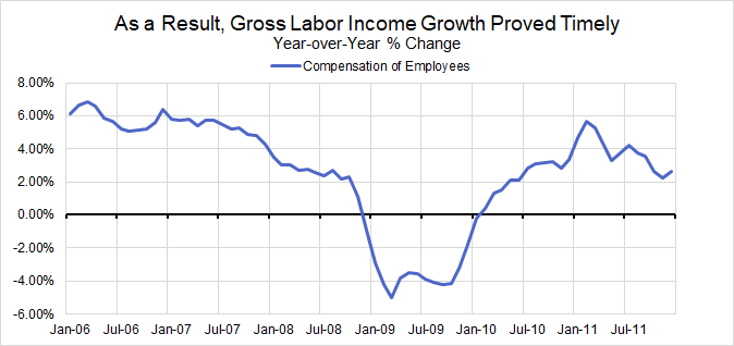
At the risk of sounding blasphemous about mainstream macroeconomic theory, consumer price inflation isn’t robust enough as an indicator to serve as the central motivation for all Fed policy decisions. Among the major sets of cyclical indicators, consumer price inflation is arguably the most disconnected and uncorrelated. Even when inflation does exhibit cyclical sensitivity, it often lags by several quarters and makes the communication of policy especially complicated if current inflation readings are at odds with more timely indicators. Finally, the methodology for calculating consumer prices is in constant flux. New price datasets and techniques for adjusting prices for quality change are regularly being introduced to an increasing share of inflation components. All of this makes it harder to disentangle what official inflation readings tell us about the current environment. GLI, which can be captured by the “Compensation of Employees” series in the monthly Personal Income release, is superior on all three counts: it is more sensitive to cyclical dynamics, it is more coincident to business cycle realities, and it follows a more stable methodology.
The Fed’s bias for tight policy is commonly framed in terms of its inability to raise inflation to its target, but aiming for higher GLI growth would also address the human cost of the Fed’s bias: forgone gains in employment and wages. By relying heavily on variables that are ill-suited for real-time estimation, such as the natural rate of unemployment and productivity, the Fed has consistently underestimated the scope for labor market progress. Instead of trying to constrain the extent to which the unemployment rate falls or wage growth rises, the Fed should use its policy tools to achieve at least a floor rate of GLI growth.
The Fed is operationally independent, but its policy commitments are only as credible as Congress permits them to be. Aiming for higher GLI growth, a function of higher employment and higher wages, is likely to garner more support from Congress than a strategy centered solely around aiming for higher inflation. The European Central Bank (ECB) and the Bank of Japan (BoJ) have shown us that despite their single-mandate objectives to raise inflation to target, political and institutional skepticism can still get in the way of optimal policy. Central banks should not be let off the hook for missing their goals, but the nature of their goals will also affect their ability to achieve them. GLI is the more appropriate benchmark for ensuring that Congress will empower the Fed to take the necessary set of actions to fulfill its dual mandate objectives, even if conventional policy is constrained at its lower bound.
In practice, GLI growth should be pursued asymmetrically, where lower GLI growth outcomes motivate a policy response in a manner that higher GLI growth alone does not. The lower the probability of GLI growth breaching its floor, the greater scope for sensitivity to inflation. Our approach would help ensure the political sustainability of the Fed’s framework and better capture the unique costs and risks associated with the effective lower bound (ELB) of interest rate policy.
Americans want a bigger paycheck, not a higher cost of living. The Fed can help.
The “Problem” Of Too Little Inflation
The Fed is facing an existential risk, one that goes beyond a replay of the Great Inflation, the Great Recession, or the current volatility in the Oval Office. At stake for the Fed is its relevance: is the institution that is tasked with managing business cycle risks well-positioned to cope with the next downturn?
The Role of Inflation Expectations
Federal Reserve Chair Jerome Powell claimed in his speech at Jackson Hole last year:
Not only are anchored expectations supposed to reinforce inflation outcomes, but they also define the most accommodative policy stance the Fed can deliver with its most conventional tool. The Federal Open Market Committee (FOMC) announces a nominal interest rate target at each Fed meeting, but the FOMC frames its policy stance in terms of a real interest rate — the difference between its nominal interest rate and the expected rate of inflation. If the lowest nominal rate that the Fed can deliver is 0% and inflation expectations are anchored at 2%, then -2% is the most accommodative real interest rate achievable.
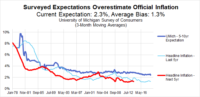
Figure 1: “Headline Inflation” uses the deflator for personal consumption expenditures. The bias is even larger if calculated with 10-year inflation rates (1.5%). Source: University of Michigan, BEA, Author’s Calculations
Figure 1 shows that long-term inflation expectations among consumers surveyed by the University of Michigan have a substantial upward bias relative to the official inflation rate. After adjusting for the bias, the most recent reading for long-term inflation expectations — a 40-year historic low in the survey’s history — implies inflation outcomes about 1% below the Fed’s target. With inflation outcomes already underperfoming the Fed’s target and expectations sliding, is the solution simply for the Fed to aim for higher inflation?
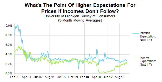
Figure 2: For the last 15 years, consumers’ short-run expectations for income growth have persistently underperformed their expectations for inflation. Source: University of Michigan
If a central bank’s attempt to increase expectations for prices was not met with a corresponding increase in expectations for income, household spending behavior might grow more cautious, ultimately undercutting the central bank’s original effort. Figure 2 confirms that the two can disconnect, and in ways that would seemingly constrain spending behavior and inflation outcomes.
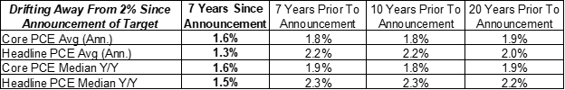
Figure 3: Headline PCE is based on prices of all goods and services classified under consumer spending. Core PCE excludes food and energy items. Source: BEA
As Figure 3 shows, the Fed’s ability to achieve 2% inflation outcomes actually diminished after the Fed’s announcement. Commodity prices fell aggressively during this period, but even after excluding the most extreme price changes, the underperformance remains visible. The absence of a recession in this seven-year period makes this persistent miss to the downside all the more glaring.
The Fed announcing its way to higher inflation might sound effective in theory, but in practice, this is a fragile strategy.
An Inferior Nominal Anchor: The Quirks of Inflation and the Superiority of Gross Labor Income
Consumer Prices Are Less Cyclical and More Idiosyncratic Than GLI
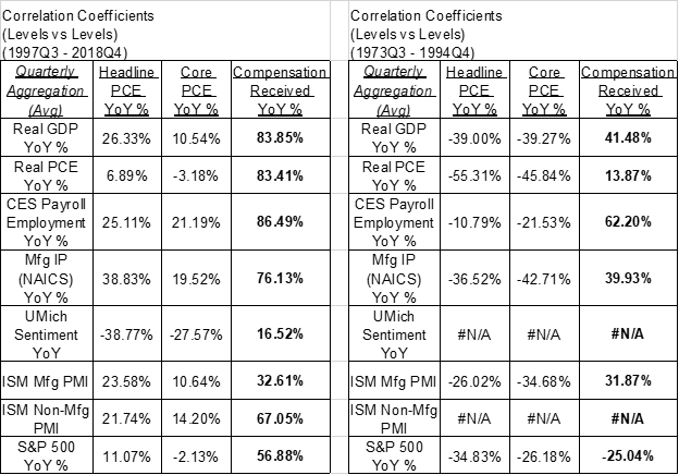
Figure 4: These correlation coefficients are based on 4-quarter changes in each of these economic indicators at a quarterly frequency. For example, the first numerical cell of this table measures the correlation between the 4-quarter change in year-over-year GDP growth and the 4-quarter change in year-over-year headline PCE inflation. 1997Q3 was chosen as the starting cutoff to the first period because that is the earliest quarter for which the ISM Non-Manufacturing PMI is available. 1994Q4 is chosen as the ending cutoff of the second period because it approximately reflects the point when long-term inflation expectations in the University of Michigan Survey begin to stabilize.
Figures 4 and 5 show that consumer price inflation is not particularly cyclical, especially in comparison to growth in GLI, as measured by the “Compensation of Employees, Received” series from the Personal Income release. GLI growth is reasonably correlated with trends in output growth, labor market activity, consumer surveys, business surveys, and financial markets. Consumer price inflation is not. There’s a temptation to attribute this stylized fact to the anchoring of inflation expectations, but it appears to hold even in periods when inflation expectations were not as clearly anchored.
Figure 5: These correlation coefficients are based on the levels of each of these economic indicators at a quarterly frequency. For example, the first numerical cell of this table measures the correlation between the level of year-over-year GDP growth and the level of year-over-year headline PCE inflation. Sources: See Figure 4
It does not make sense to put more weight on a lagging variable when monetary policy, still near the zero lower bound, will need to act swiftly if risks of significant downturn emerge.
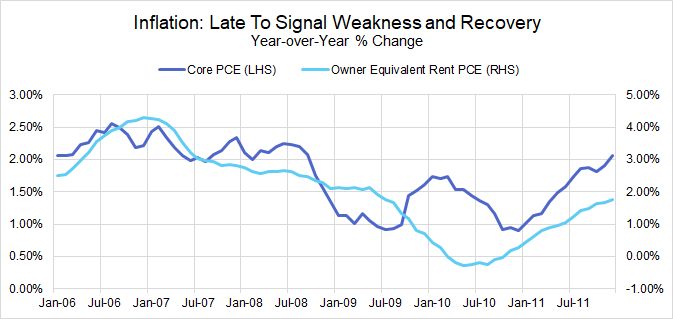
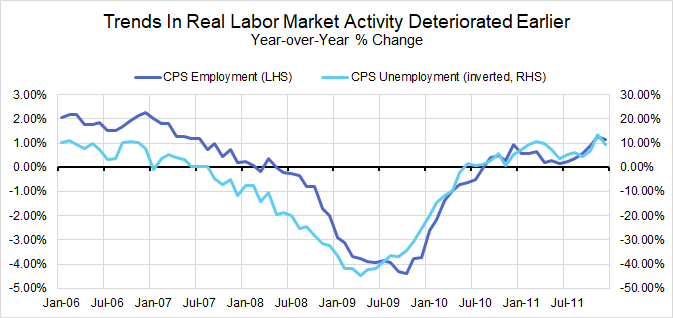
Inflation tends to lag even more than labor market indicators, in part because of a quirk in how rent components, which make up nearly a fifth of core PCE, are measured. Estimates of individual wage growth, such as average hourly earnings and the employment cost index, can also lag or be distorted by measurementissues. Nevertheless, employment and unemployment indicators in the Current Population Survey (CPS) can be especially useful for tracking and projecting GLI growth dynamics, as seen in Figures 7 and 8.
The summer of 2008 is perhaps the most glaring example of how inflation lags. Core and headline inflation were running above 2% even though other nominal and real measures of activity suggested a deteriorating economic trajectory. In each of the past three recessions, inflation troughed well after labor market activity measures. Even in non-recessionary periods such as 2011, rising inflation was ultimately a sideshow relative to the economic deceleration and elevated recession risk that policymakers needed to head off.
Forward-looking monetary policy might be the theoretical solution to dealing with inflation’s lagging property, but in practice, the lag just makes policy more difficult to communicate. In both 2008 and 2011, rising inflation seemed to motivate an elevated market expectation for policy tightening, even though the Fed subsequently chose to ease policy further in both instances. A timelier nominal anchor for episodes involving downside risk would make it easier to communicate policy effectively.
The Fed’s Nominal Anchor Should Follow A Stable Methodology
One of the underrated advantages of focusing on GLI is that the definition is largely stable, whether you rely on the estimate from the Personal Income release or the Current Employment Statistics (CES) survey. In this regard, GLI is also superior to nominal GDP, which could also prove sensitive to methodological changes.
Fixing The Fed’s Real Shortcoming: Forgone Gains In Employment And Wages
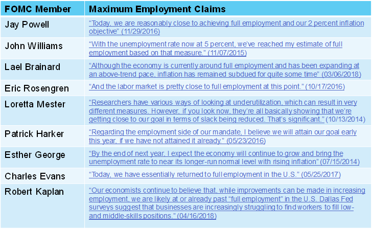
False Definitions of “Maximum Employment”
The underperformance of inflation has led FOMC members to see themselves as failing mostly on the “price stability” side of their dual mandate. We would urge against taking such a narrow perspective. While FOMC members largely sound content with the current state of the labor market, persistent errors in their evaluations suggest that a deeper revision of priors is now necessary.
Back in February of 2015, then San Francisco Fed President John Williams claimed in a Financial Times interview:
Since President Williams’ claims of achieving maximum employment, another 8 million jobs have been created. The unemployment rate has continued to fall, now to 3.6%, without much sign of inflation sustainably accelerating through the Fed’s target.
Figure 10: Source: Federal Reserve System, New York Times, Wall Street Journal
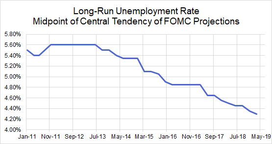
Figure 10 shows that President Williams was hardly alone in his assessment, nor has this type of error proven to be especially unique among FOMC members in recent years. To the extent that a natural rate of unemployment exists in the long run, FOMC members have collectively and consistently overestimated it. In the last 24 releases of the FOMC’s Summary of Economic Projections, 13 releases revealed a downward revision to the central tendency of the Committee’s longer-run unemployment rate projection. Not once in this period did we see an upward revision. In total, the longer-run unemployment rate has been revised down from 5.6% to 4.3% in the past 5 years, and seems poised to fall further.
Figure 11: Source: Federal Reserve System
Beware of the Problems With The Unemployment Rate
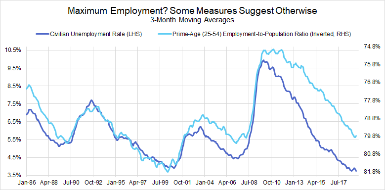
Recent research also suggests that the unemployment rate is a flawed proxy for gauging additional labor supply available. Ahn and Hamilton (2019) show that the distinction between those who are unemployed and those who are classified as not in the labor force is not well-defined within the CPS, and it tends to result in an underestimation of both the unemployment rate and the participation rate. The prime-age employment-to-population ratio, while imperfect in its own ways, was more robust to these muddy definitional distinctions. A more careful look at Figure 12 would suggest that members’ claims of achieving “maximum employment” were far too hasty.
Figure 12: The prime-age employment-to-population ratio is a broader measure of labor market slack than the unemployment rate because it does not make strong distinctions between those who are unemployed and those who are not officially participating in the labor force. Focusing on the prime working-age cohorts (25–54 year olds) helps adjust for different labor force participation trends among certain age segments (e.g. the oldest and youngest cohorts are least likely to participate). Source: BLS
Underrating “Sustainable” Wage Growth
Not only did FOMC members underestimate the number of people who could be employed without threatening price stability, they were also too cautious about the wage gains that could be achieved. In his first Monetary Policy Report to Congress in early 2018, Chair Powell noted:
Innocuous as these remarks might appear, they do reveal skepticism about just how much wage growth could prove sustainable amidst low observed productivity growth. At the time of Chair Powell’s testimony, unit labor costs, which should adjust wages for productivity, were growing faster than 2%. If low productivity growth persisted, shouldn’t faster unit labor cost growth ultimately result in a corresponding price adjustment, thereby creating above-target inflation?
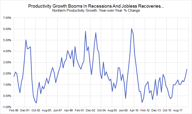
Here’s the catch: productivity is notoriously difficult to estimate in real-time, and particularly difficult to use for the purposes of policymaking. Figure 13 shows that short-run changes in the productivity data now tend to move countercyclically. When businesses decide to aggressively shed or hire labor, output per hour estimates will be driven primarily by the denominator, hours worked.
Figure 13: The strongest years for productivity growth (1992–93, 2002–03, 2009–10) have all been years where employment was declining but output growth was beginning to recover. Source: BEA
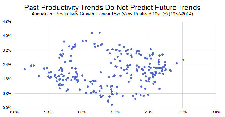
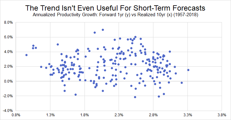
There is also little evidence that the realized long-term trend in productivity growth can predict future productivity dynamics. Whether it is for the next 5 years or just the next 4 quarters, Figures 14 and 15 highlight the dangers of extrapolating past productivity trends into the future. At the very least, it should not serve to constrain future wage growth when there is little evidence that past productivity gains have flowed back to workers.
Figure 14: Source: BEAFigure 14: Source: BEA
There are also conceptual issues associated with how productivity is measured. Do our estimates sufficiently adjust for quality improvement and capture the full scope of productive activities? The implications of higher unit labor costs for consumer prices are equally tenuous. Perhaps firms are willing to accept some short-term loss of profit margin due to competitive pressures or a pursuit of greater market share.
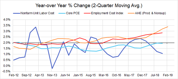
Figure 16: Since 2017Q4, unit labor costs growth has again corrected down while measures of individual nominal wage growth have continued to slowly accelerate. Source: BEA, BLS
Above all else, the evidence of an empirical relationship between unit labor cost growth and consumer price inflation is unimpressive. Look no further than the past couple of years in Figure 16. Despite unit labor cost growth exceeding 2% in the latter half of 2017, core inflation did not exceed the 2% target and measures of wage growth have still continued to accelerate. Higher wage growth was more sustainable than previously perceived.
Remove The Artificial Ceilings on GLI Growth
How necessary is it for the Fed to impose additional constraints on what the labor market can achieve? Such constraints are of empirically questionable value. Gust, Lopez-Salido, and Meyer (2017) show how such constraints can actually prove counterproductive to the Fed’s goals once the unique costs of the lower bound are fully appreciated.
Instead of embedding artificial ceilings, the Fed should aim to achieve at least a floor rate of GLI growth. The holistic nature of GLI means that the Fed does not have to be particularly precise about whether gains come from unemployment rate declines, participation rate increases, or wage acceleration. The Fed has every reason to act as as a tailwind to the American worker, not an additional headwind.
Ensuring Credibility When Constrained: Aligning The Framework To Popular Desires
Central Banks Do Not Operate Within A Political Vacuum
In order for central banks to maintain their independence in democratic societies, it is important that they continue to pursue democratically desirable goals. If higher inflation becomes the sole focus of the Fed’s strategy, Congress might take a skeptical view, even though such a strategy could prove consistent with more obviously desirable outcomes. The Fed’s policy commitments are only as sustainable and credible as Congress allows them to be. Aiming for higher GLI growth, a function of higher employment and higher wages, is likely to garner stronger support from Congress.
Just 8 years ago, the Fed was at a fragile point in the post-crisis expansion. Compensation growth and other labor market measures were already slowing visibly by the second quarter of 2011, but, as Figure 17 shows, inflation was continuing to pick up.
Given the macroeconomic conditions and the constraints around monetary policy in 2011, switching to a regime that explicitly promised elevated inflation would have proven advantageous for achieving the dual mandate. Unfortunately, it may have resulted in even more political pushback. While no framework would have been a universal crowd-pleaser in that moment, an explicit commitment to fattening the nation’s paycheck would have stood a better chance of navigating such rough political waters.
Studying Abroad: Institutional Frictions Hindering Central Banks’ Ability To Raise Inflation To Target
We can also learn from the experiences of the ECB and the BoJ. The challenges of the lower bound coupled with their institutional and political constraints have resulted in an inability to achieve their inflation goals. Such constraints have hindered their willingness to promptly use unconventional tools in order to raise inflation to their targets.
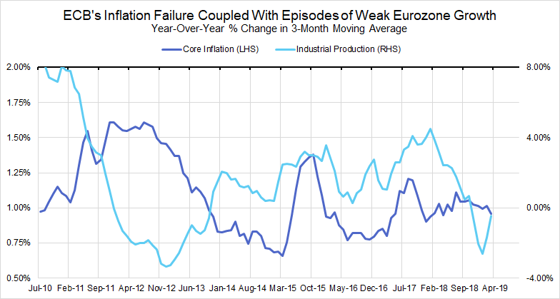
Since the global financial crisis, each time the Eurozone has been hit with a downside cyclical shock, the shadows of German policymakers have loomed large. The ECB’s mandated goal since 2003 has been “to maintain inflation rates below, but close to, 2% over the medium term.” This should have meant a symmetric approach to achieving inflation outcomes near 2% and a willingness to brush off transitory effects. Unfortunately, a mandated goal does not always mesh with existing political realities.
Deteriorating financial conditions, historically elevated unemployment, and slowing growth would generally offer enough reasons for a central bank to consider easing policy. Yet in the middle of 2011, former Bundesbank president Axel Weberwas successful in advocating for the ECB to pivot from policy easing to policy tightening. His key point of persuasion? Higher commodity prices! Meanwhile, core inflation measures were still missing the ECB’s inflation target and the Eurozone fell into a historic recession and financial crisis soon after. So much for “over the medium term.”
No framework is going to fully satisfy dogmatically hawkish policymakers and constituencies. Nevertheless, a robust framework can help put central bankers in a better position to withstand and counter such criticism as they pursue the optimal policy.
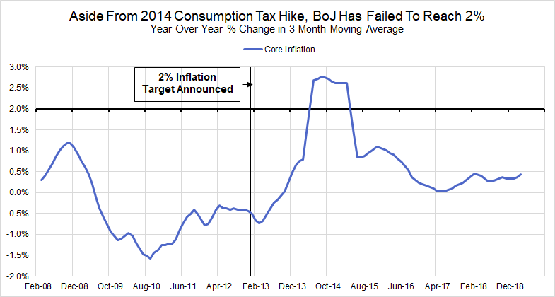
Japan has observed persistently low and often negative inflation rates for the past 25 years, but the political will to address it as a problem only emerged in December 2012 with the election of Shinzo Abe as Prime Minister. Since that time, the Bank of Japan has engaged in an ambitious strategy to achieve the singular goal of sustainably raising inflation to 2%. Unfortunately, the results suggest that the strategy has still failed to achieve its objective, and now the motivation for achieving the 2% target has faded. The Financial Times reported on a recent statement from BoJ Governor Haruhiko Kuroda:
With core inflation still running well below the 2% inflation target, has the situation actually changed so meaningfully that Governor Kuroda can make such a claim?
Figure 19: Core Inflation excludes fresh food and energy. Source: Ministry of Internal Affairs and Communications
Figure 19 would suggest that the situation has not changed that drastically. Governor Kuroda’s reduced ambition seems to have less to do with any improvement in economic circumstance and more to do with the erosion of political will. Bloomberg reports:
Preparing For (And Preventing) The Next War At The Lower Bound
A discussion of the Fed’s framework is not the same as a discussion of its toolkit, but the two are clearly intertwined. If conventional policy is at the lower bound, what is the right intermediate target for ensuring that Congress will empower the Fed to use the necessary tools to fulfill the objectives of the dual mandate? This framework review can go a long way to putting the Fed in a stronger position to provide necessary accommodation in such scenarios. If the economy is in trouble and the policy rate is already at the lower bound, the pursuit of higher GLI growth is going to offer a better justification to Congress for using unconventional policy tools.
As the ECB and BoJ are currently showing us, the lower bound of conventional monetary policy creates a variety of new problems and costs that are omitted within standard macroeconomic models. We still do not know if the unconventional policies developed since the financial crisis are sufficient to achieve the dual mandate. By taking steps to continuously ensure a baseline floor under GLI growth, the suggested framework would give the Fed a better chance of acting preemptively to avoid protracted downturns before running out of policy tools.
The Mechanics of Our Framework: When and How To Support Gross Labor Income Growth
Policy Rules For Understanding The Reaction Function
GLI, like consumer prices and nominal GDP, can be placed within policy rules in ways that still satisfy mainstream macroeconomic principles. Our recommended reaction function, specified in Figure 20, is a combined version of two forward-looking first-difference rules in forms similar to what is suggested in Orphanides and Williams (2008, 2013). Assuming forecast certainty, the “CF Rule” takes on a discontinuous property that addresses the asymmetric nature of the “maximum employment” objective. Low GLI growth is a reason for easier policy, but high GLI growth does not necessarily demand tighter policy.
Figure 20
Accounting for Forecast Uncertainty…Asymmetrically
Of course, assuming forecast certainty would be very unrealistic. By taking a more probabilistic view of the projected outcomes, we can derive a more continuous policy rule that still pursues “maximum employment” asymmetrically. In the “UF Rule” in Figure 20, the probability of GLI growth breaching its floor is pivotal to the reaction function. The higher the likelihood of falling short of the GLI floor, the greater the relevance of GLI growth projections for policy decisions. The lower the likelihood of falling short, the greater the relevance of inflation projections.
The rule under forecast uncertainty intentionally encourages faster and sharper reaction to the risk of major downside shocks. The Fed would be better-positioned to react promptly, thereby reducing the risk of doing too little, too late and hopefully avoiding the challenges associated with conducting policy at the lower bound.
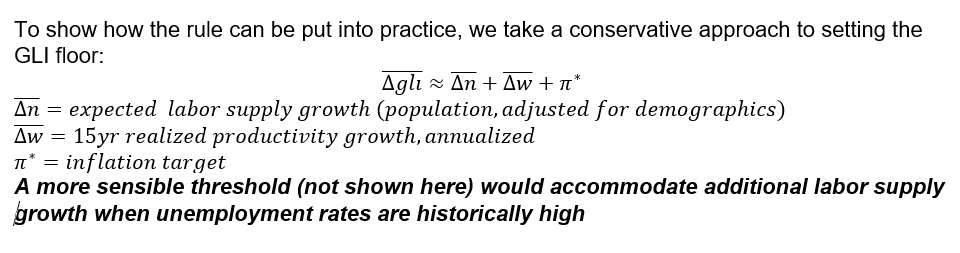
A Conservative Method For Setting The GLI Floor
GLI growth is a function of labor supply growth, real wage growth, and inflation. A conservative approach to setting the labor supply growth component of the threshold would only include a demographic-adjusted estimate of working-age population growth, as will be shown in upcoming examples. A more fair-minded approach would also allow for additional employment growth in periods when the unemployment rate was relatively high.
Real wage growth is supposed to be consistent with productivity growth, but the full extent of productivity gains are often only revealed after the fact, in the weakest moments of labor market activity. The realized productivity gains in recessions and jobless recoveries have not made their way back to labor compensation, or else we would not see such a historically depressed labor share of income. So while it is not a good reason to constrain future wage outcomes, a realized long-term productivity trend that spans a full business cycle can still serve as a reasonable baseline for real wage growth.
The inflation component of the threshold should simply be the Fed’s inflation target over the medium-run. Figure 22 shows that the GLI floor should now be at least 4.1%growth year-over-year, as measured by the “Compensation of Employees” series.
Figure 22: The labor supply growth component is derived from local trends in prime-age (25–54) and non-prime-age (not 25–54) employment rates and population growth (currently 0.7%). The real wage growth component is equivalent to the 15yr annualized rate of nonfarm productivity growth (currently 1.44%). The inflation target embedded in this threshold is 2%. Keep in mind that FOMC views on the appropriate inflation target have not always been 2%.
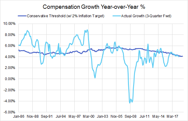
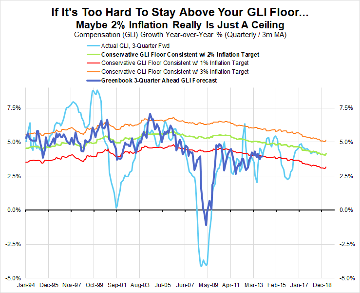
Targeting The Fed’s Compensation Growth Forecast
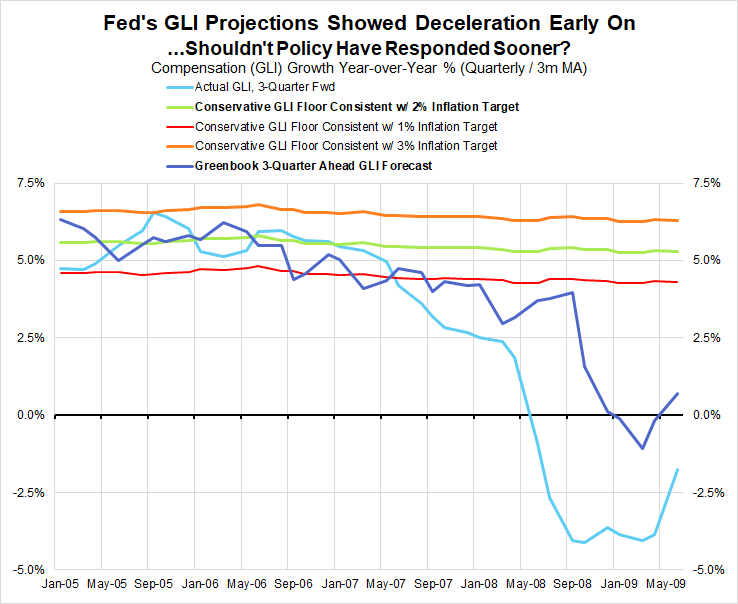
As shown in Figure 23, the Fed’s Greenbooks can help us derive an as-reported time series of GLI growth forecasts. The Fed staff at least implicitly forecasted GLI growth at each FOMC meeting because it regularly forecasted (nonfarm) compensation per hour growth, (nonfarm) output per hour growth, and aggregate output (GDP) growth.
Figure 23: “Conservative Floor” refers to the fact that the floor does not assume additional labor supply gains when estimates of labor market slack are elevated. Labor supply growth is solely a function of trends in population growth and demographic structure. Source: Federal Reserve System, BEA, BLS
There are minor issues associated with mixing nonfarm and aggregate measures and adjusting for the opaque policy assumptions that underlie these forecasts, but the forecasts used in this exercise should not be particularly sensitive to these issues. The approach to using the Fed staff’s forecasts is consistent with the approach in Chair Bernanke’s January 2010 speech for working with forward-looking Taylor Rules.
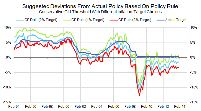
By using the rule in Figure 20 that (unrealistically) assumes forecast certainty, we can compare the rule’s prescriptions under a variety of inflation target assumptions with what actually transpired, as shown in Figure 24.
Figure 24: The coefficients on GLI growth and inflation are approximated using the nominal income targeting rule in Hendrickson (2012) and a forward-looking first-difference rule in Orphanides and Williams (2008). “CF Rule” refers to the policy rule that ascribes full certainty to the Fed staff’s forecasts (yes, this is unrealistic).
The Descent Into The Great Recession (2006–08)
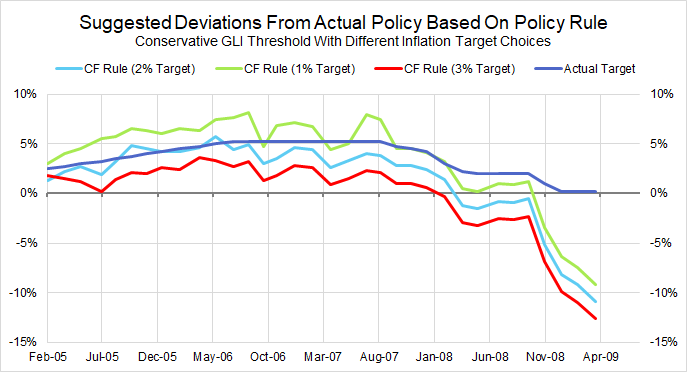
Figure 25: Only when GLI growth projections broke through the floor consistent with 1% inflation did we see the Fed begin easing (September 2007).Figure 26: The persistence of such low GLI growth projections suggested, as per the rule, that easing measures needed to be introduced earlier and more persistently until projections converged back to the GLI Floor.
Based on the conservative estimate of the GLI floor that incorporated a 2% inflation target, Figures 25 and 26 show that policy easing would have begun as early as the June 2006 meeting because of the Fed’s deteriorating projection for GLI growth. Contrast this with the actual June 2006 meeting, when the Committee voted for its final rate increase of the 2004–2006 tightening cycle. If a 1% inflation target was assumed instead, projections for GLI growth would have only begun falling persistently below the GLI floor in September 2007. It is a dumb coincidence, but this meeting was when the FOMC actually began easing. Despite the elevated rates of inflation in 2007 and 2008, the costs of the Great Recession and the financial crisis now show us that it was still better to err on the side of easing earlier and faster in this period.
Tightening During A Jobless Recovery (2009–10)
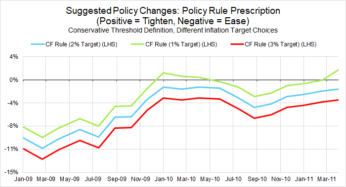
Figure 27: A GLI floor that embedded a 2% inflation target would have prescribed more persistent easing. A 1% target would have prescribed modest policy tightening in the first half of 2010.
At that time, GLI growth was projected to be roughly 4.5%-5%, a sharp rise from previous projections but hardly impressive in the context of population growth and historically high unemployment. Even under the conservative specification of the GLI floor that assumed a 2% inflation target but ignored high unemployment, our framework would have still prescribed additional easing. Policy tightening under our approach would have required a GLI floor with a much lower assumption for the inflation target, closer to 1%, or a lower threshold for real wage growth.
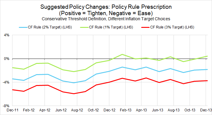
Figure 27: The CF Rule that includes a 2% inflation target would have prescribed continued policy easing throughout 2013. Whether the taper tantrum qualifies as tightening or merely the end of easing, the preference for the taper aligns more closely with a 1% inflation target under our approach.
Even if we look exclusively from the period subsequent to the 2% inflation target announcement in January 2012, the urgency in 2013 to taper asset purchases would be puzzling under our suggested reaction function. For the end of additional easing to be justified, the threshold would need to incorporate some combination of a lower inflation target and a lower threshold for real wage growth.
Extracting The Advantages of Level Targeting While Avoiding Its Drawbacks
This framework can also incorporate a level targeting strategy, which seems appropriate on a temporary basis if policy tools are of diminished capacity or reliability, as was the case during and after the financial crisis. A level targeting approach in these instances would ensure that if GLI growth underperformed the floor, the Fed would aim for faster GLI growth in subsequent periods.
Nevertheless, a permanent level targeting strategy using GLI does face some practical challenges. The first is simply a matter of false precision. Aiming to achieve a certain rate of growth is challenging enough, but to achieve a pre-defined set of levels makes policy especially sensitive to one-offs. Transitory dynamics may otherwise prove irrelevant over the medium-run but could distort the policy response under a level-targeting strategy. In the case of GLI, there is some scope for short-term distortion if tax laws are expected to change, as they were during the fiscal cliff negotiations of 2012.
The second challenge with permanently adopting a level-targeting strategy relates back to the asymmetric preferences surrounding GLI as a benchmark. While it is reasonable to see why insufficient paycheck growth deserves some “catch-up,” we do not think outperforming paycheck growth, as was the case in 1999 or 2000, deserves “catch-down” policy tightening.
Concluding Thoughts
The Fed’s ongoing review of its framework is a great opportunity to correct some of its persistent mistakes and recommit to the goals expressed in the Humphrey-Hawkins Act.
Now is not the time for tinkering at the margins of inflation targeting. To rectify its more glaring and costly errors, the Fed needs to focus on supporting GLI growth. GLI is a better nominal anchor than consumer prices for reflecting downside cyclical risks in a timely manner. By ensuring sufficient GLI growth, the Fed will be less distracted by faulty estimates of labor market constraints, and more focused on fulfilling its mandate to maximize employment. Ultimately, supporting GLI growth will politically empower the Fed to pursue policy that is both optimal and popular, which could prove helpful if the Fed needs additional policy tools or credibility to reshape expectations.
In more recent decades, the major macroeconomic problem has been one-sided and suggests that monetary and other macroeconomic policies have been systematically too tight. High wage growth and high price inflation have become exceedingly rare, while contractions in employment have been protracted. The mechanics of the GLI floor within our framework offer a straightforward correction.
The FOMC and the Fed staff has never been better-positioned to get this right. Americans want more growth in their paychecks, not a higher cost of living. The Fed can help. The Fed should help.
The link has been copied!
Your link has expired. Please request a new one.
Your link has expired. Please request a new one.
Your link has expired. Please request a new one.
Great! You've successfully signed up.
Great! You've successfully signed up.
Welcome back! You've successfully signed in.
Success! You now have access to additional content.