Executive Summary

The Implications of the Fed’s Framework Revisions For The Fed’s Communication of Maximum Employment:

Given the Fed’s recent framework revisions and forward guidance commitment to maintain current interest rates until “maximum employment” is achieved, the Fed’s communication with respect to its assessment of “maximum employment” is overdue for a clarification. The previous framework hardwired the Phillips Curve into the Fed’s approach to setting interest rates, with the belief that the unemployment rate had to always be landed on a pin, not too high, not too low, if inflation was to stay well-behaved around the 2% target. The Phillips Curve has always been on shaky footing empirically, but the Fed’s new asymmetric approach — only easing to address employment shortfalls — removes a long-standing policy-induced ceiling on labor market possibilities.

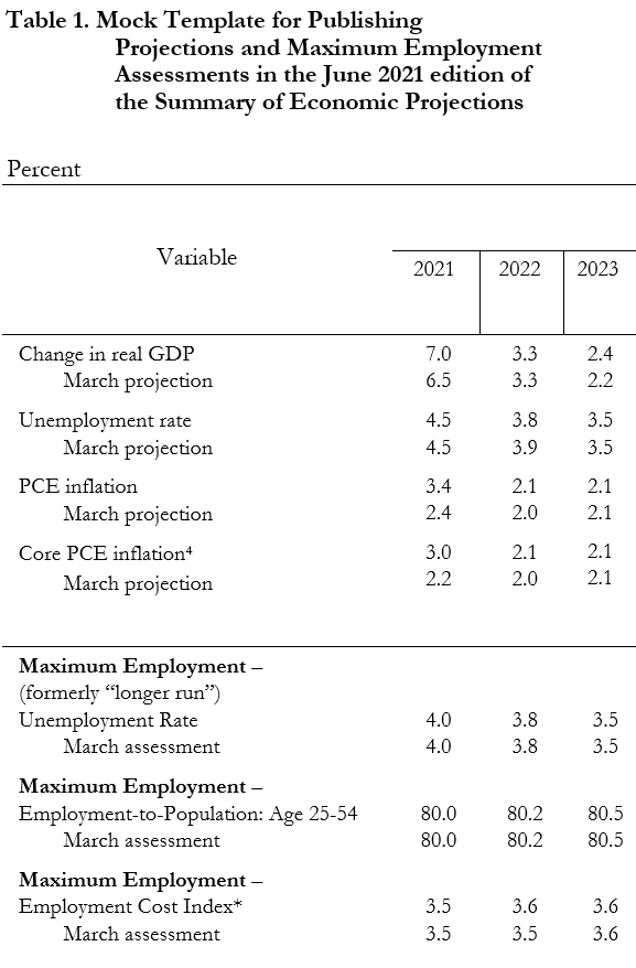
The Summary of Economic Projections is still structured with the Fed’s old framework in mind. Maximum employment is only publicly assessed with a single indicator — the highly flawed unemployment rate — and at a single, abstract point in time — when unemployment declines and general labor utilization gains are presumed to stall out at a fixed level. To orient policy around that imagined equilibrium is to ignore the basic empirical fact that stalling labor utilization rates tend to correlate with business cycle fragility, while new labor utilization peaks generally do not appear to have persistent inflationary consequences.

The Fed’s approach to communications is essential for correctly translating their desired set of policies and objectives into financial conditions. When the Fed’s views as to what path financial conditions must follow to support a strong labor market diverge from the market’s, it is the market’s view that will prevail on financing conditions and private sector risk appetites. Unless the Fed can resolve these public communications issues, they will have no assurance that their policies will take hold and succeed.

The Tradeoffs Between Maximum Employment and Stable Prices are Time-Varying and Context-Dependent

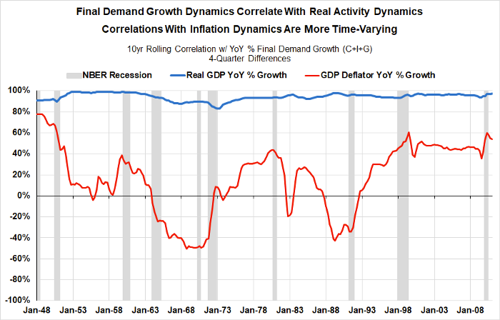
Interest rate policy affects financial conditions, which in turn can support nominal spending and real economic activity. Periods of high growth in nominal spending and real activity tend to be locally correlated with faster rates of labor market progress for fairly straightforward reasons. The extent to which such periods have inflationary consequences is a more difficult question, which requires a more granular evaluation of capacity in particular sectors and yields more time-varying and context-dependent answers. Evaluation of capacity constraints requires a more disaggregated view of capacity. It also requires an assessment of the time and investment needed to sustainably ease inflationary pressure and accommodate current demand.

The evaluation of capacity constraints should not be confused with a sticky level of labor utilization that the logic of the Phillips Curve embodies. Whereas the implications of capacity constraints necessarily involve granular estimations in specific sectors, labor utilization is a simplified aggregate of physical hours worked or employed persons. Labor utilization can be relatively high even as capacity constraints fail to meaningfully bind. Labor utilization can be relatively low even while capacity constraints are widespread.

Scenarios That The Fed Should Be Well-Equipped To Communicate:

To avoid such confusion, the Fed must be able to communicate dynamic assessments of maximum employment that grapple with a wider set of scenarios than its previous framework was able to handle.

1. 2015–2019: The Incoherence Of Going “Beyond Maximum Employment” Maximum employment can evolve and expand over time in a way that a unitary projection will miss; such progress should be welcomed.
2. 2004–2006: Multi-Year Inflationary Dynamics May Imply Temporary Speed Limits, But Not Permanent Destination Limits. Inflationary dynamics can sometimes persist — even over a multi-year period — thereby constraining the feasible pace of progress, but such dynamics should not make the ultimate destination of full employment impossible to reach. Short and medium run constraints to employment imposed by inflationary pressures should be disentangled from the longer run possibilities for labor utilization.
3. 2009–2012: Resisting Recessionary Revisions That Re-classify Cyclical Employment Shortfalls As Structural. Asymmetric treatment of labor market outcomes should imply upwardly mobile assessments of maximum employment that are still downwardly sticky to recessionary shocks.

We provide a template here for communicating the dynamic nature of maximum employment estimates, with ample room for assessing maximum employment across multiple indicators, including labor utilization and wage growth, to ensure robustness. Dynamic assessment necessarily involves iterative revision of maximum employment assessments. Dynamic assessment also involves revising the set of indicators that best reflect how the maximization of the workforce’s potential compares with current employment. We hope to see the Fed take a similar approach in how they choose to assess and communicate the implications of their “maximum employment” forward guidance.

The Fed’s Framework and Forward Guidance Warrant A Communications Revamp of “Maximum Employment”

Throughout the pandemic, the Fed has shown a welcome focus on “maximum employment” by treating labor market outcomes as an equal partner to price stability, as its congressional mandate requires. The Fed’s recent framework review abandons a hard 2% inflation ceiling for an Average Inflation Targeting regime, while the September 2020 forward guidance conditions any future rate hikes on the achievement of “maximum employment,” whether or not inflation floats past 2%. This approach leaves more room for non-inflationary labor market progress than prior policy stances. Chair Powell drove this point home in March, acknowledging that “4% would be a nice unemployment rate to get to, but it will take more than that to get to maximum employment.”

All of this — the framework review, the forward guidance, statements by FOMC members — stands in healthy contrast to the hawkish approach after the Global Financial Crisis. Although the Fed used the same tools of low rates and forward guidance, it conditioned rate hikes on the achievement of a much more modest 6.5% unemployment rate. Rather than pursue “maximum employment,” the Fed seemed wedded to the conceptual framework of the Phillips Curve, which claims that labor markets tighter than a specific level of labor utilization always and everywhere create excess inflation.

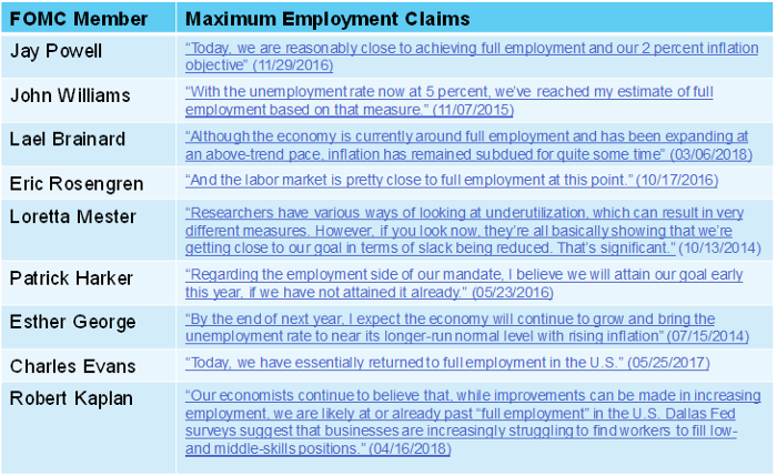
While this newfound focus on labor market outcomes is admirable, the Fed’s leadership has yet to explain what labor market conditions are consistent with their estimate of “maximum employment.” Without clarifying this crucial component, the Fed risks substantially miscommunicating its reaction function. So far, the only clue the Fed’s current communication strategy provides is the FOMC’s longer run projection of the unemployment rate, the rate deemed to be consistent with its Congressionally mandated objectives.

On its own, this approach is unsatisfactory. The unemployment rate is a deeply flawed metric for proxying labor utilization. Underlying the rate is an assumption that one can neatly distinguish between the unemployed and those who are not participating in the labor force — but the Current Population Survey does not have that capability. Thankfully, better metrics do exist.

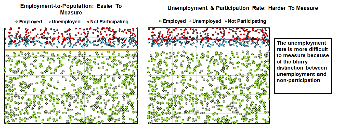
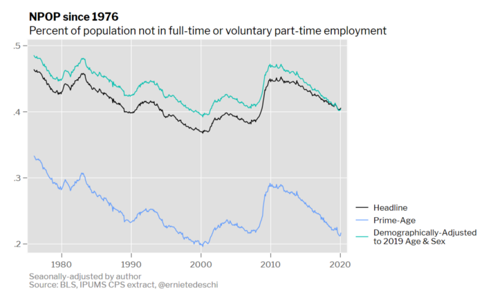
The prime-age employment-to-population ratio and Ernie Tedeschi’s NPOP measure are both strictly superior alternatives to the unemployment rate, since they suffer from far less measurement ambiguity. Both prime-age EPOP and NPOP rely on the more robustly estimated distinction between employment and non-employment (NPOP also accounts for involuntary part-time employment). It is clear when someone is or isn’t working, but far less clear when someone who isn’t working is or is not participating in the labor force.

When flaws in the unemployment rate as a metric are pointed out, FOMC members do clarify that they evaluate maximum employment on a variety of indicators. Unfortunately, these indicators — and the FOMC’s thoughts on them — are not made available to markets or the public in a systematic manner.

Worse, the “longer run” unemployment rate projection presumes the existence of a single level of labor utilization which, once reached, will be forever consistent with the Fed’s inflation target. In this imaginary longer run, employment growth is assumed to revert to population growth, adjusted for demographic changes. Effectively, age-adjusted employment-to-population ratios are assumed to stall out around a fixed level.

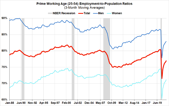
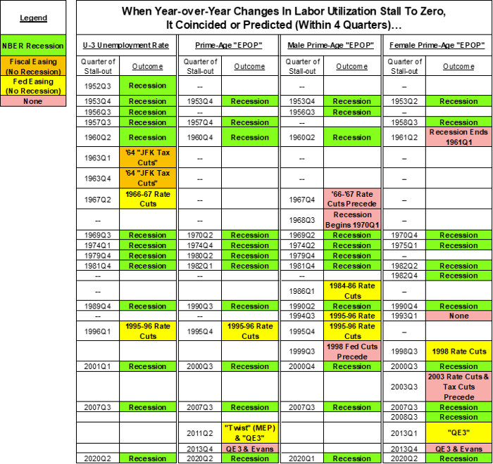
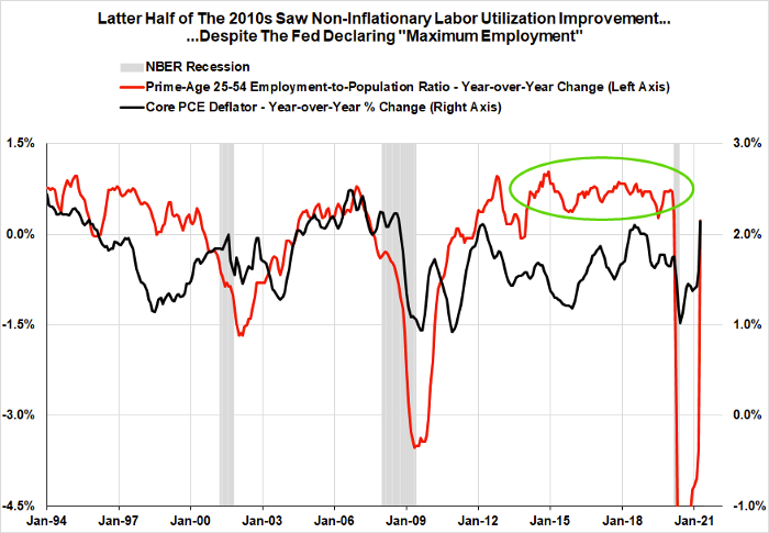
In the real world, the moment labor utilization stops rising, policy must intervene or else a recession is all but inevitable. With very few exceptions, the quarter in which progress stalled out on the unemployment rate or the prime-age 25–54 employment-to-population ratio (aggregate, male, or female) coincided with or predicted either a recession or major anti-recessionary policy intervention.

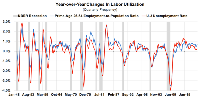
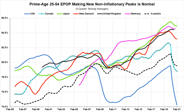
The long run static equilibrium approach also appears at odds with the experiences of other advanced economies. Many developed countries have been able to consistently push age-adjusted employment-to-population ratios to new heights without adverse consequences. Labor utilization does not simply level off at some historically established peak, and the achievement of new peaks does not coincide with persistent above-target inflationary pressures.

If policymakers and market participants are to have a better understanding of the policy tradeoffs that actually exist at a given moment, the first requirement is a clear understanding of the dynamic and multi-dimensional nature of “maximum employment.” Simply relying on metrics like the “long run unemployment rate” obscures, rather than reveals, the economic possibilities available in the present.

The risk from such a static one-dimensional approach to communicating maximum employment is that market participants and the broader public start to assume that the Fed’s relative hawkishness or dovishness will turn on the achievement of a single indicator. The Fed repeatedly tried to communicate in 2013 that the Evans Rule’s 6.5% unemployment rate condition was to function as a basic threshold condition, not a mechanical trigger for subsequently hiking interest rates. A stray comment from Chair Bernanke about tapering bond purchases when the unemployment rate came close to the Evans Rule threshold proved to be a powerful spark for the “taper tantrum” and a needless slowdown in a still-depressed housing sector.

Communications are the pipes by which the Fed’s policies translate into real economic effect. Market participants are already on the edge of their seats with the release of every new iteration of the Summary of Economic Projections. As long as the Summary of Economic Projections (SEP) codifies the logic of the Phillips Curve and static equilibrium in a bad labor utilization metric, it risks undermining the intellectual strides the Fed has taken in its recent framework review and forward guidance policies.

Tradeoffs Between “Maximum Employment” and “Stable Prices” Change With Context and Over Time

From a legal point of view, Section 2A of the Federal Reserve Act specifies “maximum employment” and “stable prices” as coequal parts of the Fed’s dual mandate. Over the years, the Fed has chosen to establish a 2% inflation target as the definition of “price stability.” “Maximum employment” has proven much more difficult to define, and approaches to its estimation swing between trivially simple measurements and ambiguous “you know it when you see it” explanations.

Some, looking to ignore the problem entirely, have defined “maximum employment” as whatever level of labor utilization obtains when the Fed hits its inflation target. If, as in the Phillips Curve, that level of utilization is presumed to be stable over time, then simple unemployment-inflation tradeoffs can mechanically guide policy. This so-called “divine coincidence” is at the heart of much conventional macroeconomic thinking: there’s no need to think about what “maximum employment” means when it can be achieved through inflation targeting alone.

If it were all this simple, we could end the piece right here. However, the tradeoffs actually relevant to the Fed’s dual mandate change over time, and are highly context-dependent.

To find and specify these tradeoffs, and make clear the stakes involved, requires something of a detour to establish how exactly monetary policy exerts control over labor market and inflation outcomes. This detour will provide us the necessary vantage point to see why inflationary pressures from capacity constraints should not be considered as an a priori indicator of unsustainable labor market tightness

Many commentators and policymakers assume there exists some direct linkage between employment, interest rates and inflation — Volcker cranked rates up and inflation went down at the cost of jobs — but the path from rates to the labor market and inflation is a circuitous one. Rates policy works directly on financial conditions, which in turn affect nominal spending and real activity, which then redound on labor market and inflation outcomes.

What we see empirically is that marginally lower interest rates support credit creation, financial intermediation and risk-appetites. These then support higher spending and incomes, which generally coincide with higher real output and consumption growth. Sustained higher real output and consumption support firm expectations of stronger flows of purchase orders and revenue, which ultimately supports increased hiring and investment. Marginally higher interest rates support the opposite forces.

However, the fact that the above is an account of general trends and tendencies means that we should exercise caution when trying to organize interest rate policy around precise relationships between labor utilization and any coincident inflationary pressures. We can be sure that if rates spike dramatically, it will have negative consequences for economic growth and employment. Nonetheless, since the path from rate policy to economic outcomes involves so many intermediate steps, interest rate policy should be treated as a blunt tool — not a precision instrument.

If we want to ask questions about what a particular rate of inflation means for the sustainability of current rates of labor utilization, we have to first understand where the inflationary pressures are coming from, and why. Without this, the specific tradeoffs that do exist become opaque, and discussion centers around the assumption that there are always direct tradeoffs between particular levels of labor utilization and inflation. It is true that there may be strong tradeoffs when current real demand exceeds current and future capacity to supply. However, the level of labor utilization tends to offer little information as to when those tradeoffs become most acute, or how to resolve them.

This state of affairs creates problems for policy analysis, as well as for traditional narratives that make inflation a function of labor market outcomes. The kinds of capacity constraints that drive inflation are never constraints across the economy as a whole (aside from the aftermath of wars). Instead, when capacity constraints bind, they often only affect a handful of key sectors. Owing to conceptual difficulties in aggregating levels of capacity utilization, these capacity constraints are rarely visible in aggregate, looking instead like low levels of utilization. The hallmark of a bottleneck is that of a few sectors running at or above capacity, while the absence of the intermediate goods those sectors produce forces many other sectors to idle plant and take capacity offline. Where this matters for our argument is that if capacity constraints are only binding in a handful of sectors, there is no good way to argue that economy-wide labor utilization is to blame.

The binding capacity constraints in energy production in the 1970s provide a clear example of how the aggregation problem matters in practice. They illustrate the importance of disaggregation and contextual assessment to understanding the relevant aspects of the supply side and identifying what tradeoffs do and do not exist for demand-side policymaking. When looking only at the aggregate industrial and manufacturing capacity utilization estimates, the era of the 1970s Great Inflation seems to coincide with much more spare capacity than the 1960s, facially at odds with the theory that capacity deficiency played much of a role in the Great Inflation.

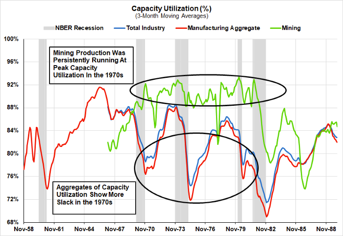
To see that there was in fact a shortage of spare capacity, you would have had to drill down into the mining capacity utilization index (which includes oil & gas extraction). Here, capacity utilization held a sustained peak for the duration of the 1970s. The inflationary pressures and input shortages elsewhere in the supply chain drove underutilization in manufacturing sub-sectors and helped create the dissonance between high inflation and low capacity utilization in the aggregate.

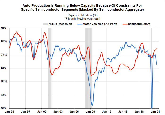
In fact, we are seeing something similar in semiconductors now. Semiconductor capacity utilization in the aggregate is still below historical peaks. However, specific segments of microchip production now face binding capacity constraints that are in turn driving underutilization in downstream manufacturing sectors like autos.

It is only by understanding the nature and rigidity of capacity constraints at a local level that the origin of certain inflationary pressures, and the consequences for different policy approaches, can be gauged. These kinds of capacity constraints say next to nothing about the aggregate level of labor utilization. Unless, that is, one is willing to make the argument that a capacity bottleneck in one sector means that all workers should earn and consume so much less that the economy as a whole shrinks to a size that can fit through the bottleneck. It is rather rare to see this position expressed.

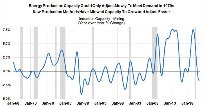
Ultimately, some capacity constraints can be alleviated by market or government actors, but others are less obliging. Despite high levels of capacity utilization in energy in the 1970s, capacity expansion was constrained by a variety of factors — new wells, transportation infrastructure, insufficient technique. This is in contrast to more recent times, when shale production methods have made capacity expansion much faster and easier when price movements signal a need. This should make clear that bottleneck sectors change with time, technology and economic organization, and policy must recognize and accommodate these changes.

The central takeaway from this detour — and a fundamental premise of our attempts to clarify how the Fed should communicate its estimates of “maximum employment” — is that inflationary pressures from capacity constraints should not be considered an a priori indicator of unsustainable labor market tightness, or confused conceptually with the idea of a sticky level of labor utilization.

In one sector, relief from capacity constraints may involve substantial time, capital spending, price increases, and engagement with non-probabilistic forms of uncertainty. In another sector, binding capacity constraints may go unnoticed by the wider economy. Whereas demand-side assessments speak the common language of dollars and cents, supply-side assessments of capacity require a murkier inquiry into each sector’s distinct relevance and linkages, something that aggregate estimates of labor market health simply cannot answer. Labor utilization can be relatively low amidst widespread capacity constraints. Labor utilization can be relatively high even as capacity constraints fail to meaningfully bind.

“It’s all time-varying” and “it’s all contextual” can sound solipsistic and somewhat depressing, but as we will show in subsequent scenarios, it need not be. Rather than a kind of nihilism, this attitude is a call to redouble our attention to the empirical facts on the ground. Some inflationary pressures resolve quickly, and some can take a while. However, the constraints these inflationary pressures reveal should be framed in terms of the speed of labor market progress, not as representing a limit to what can be achieved in the long term. The Fed’s revised framework and forward guidance has the potential to yield tremendous benefits — but these may not be achievable as long as their communications reflect a static view of maximum employment.

Three Scenarios The Fed Should Be Well-Equipped To Communicate

A core motivation for clarifying the complexity of “maximum employment” is to help policymakers prevent avoidable policy errors. From today’s vantage point, there are three scenarios where the Phillips Curve orientation has proven particularly misleading and where an appropriately dynamic approach can directly improve policy outcomes.

1. 2015–2019: The Incoherence Of Going “Beyond Maximum Employment”
2. 2004–2006: Multi-Year Inflationary Dynamics May Imply Temporary Speed Limits, But Not Permanent Destination Limits
3. 2009–2012: Resisting Recessionary Revisions That Conveniently Re-Classify Cyclical Employment Shortfalls

2015–2019: The Incoherence Of Going “Beyond Maximum Employment”

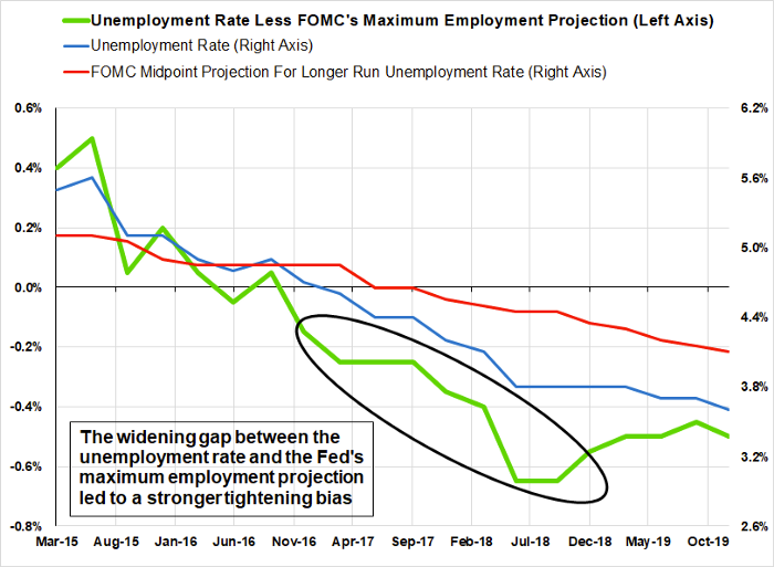
The Fed’s newfound willingness to treat employment outcomes asymmetrically comes in part from the FOMC’s late-2010s assessments that we were “beyond maximum employment,” which proved successively and persistently incorrect. Had the Fed been willing to revise its estimate of “maximum employment” upwards against a backdrop of low inflation, it could have easily avoided unnecessary policy tightening. While there is less risk of the Fed repeating this error in the near term, as the post-pandemic recovery plays out, the Fed does need to communicate clearly that it will not, on a longer timeline, repeat its earlier mistake.

Despite the unemployment rate falling below the Fed’s assessment of “maximum employment,” above-target inflation persistently failed to materialize. Almost every month, the unemployment rate would edge down and drive a wider gap between current labor utilization and what the FOMC judged to be the maximum level of labor utilization consistent with its 2% inflation target. All else equal, this is a dangerous situation according to a Phillips Curve-based approach. In that model, the widening gap between current and maximum labor utilization predicts substantial price acceleration and even suggests the possibility that inflation may suddenly spike to “where it should have been.”

Instead, inflation remained trapped below the Fed’s 2% target during this period supposedly so far “beyond maximum employment” as to warrant tighter monetary policy. The Fed apparently believed that relatively low levels of unemployment were, by themselves, enough to set off future inflation risks and justify policy tightening.

Against indications that it provides a poor guide to policy, true believers in the Phillips Curve now hide behind the notion that the curve is merely “flat,” a fancier way of saying evidence of a Phillips Curve relationship has vanished. Judging from the regional cross-section of component and aggregate price indices, the Phillips Curve has always been “flat.”

Were it not for Chair Powell’s substantial reversal of policy tightening, it is not hard to imagine 2019 as a replay of 1999–2000, when the Fed was similarly motivated to hike rates because of a low unemployment rate (despite the absence of inflationary pressures).

By adhering to “sticky” views about the location of maximum employment, the gap between where the non-inflationary labor market was and the Fed’s own assessment of maximum employment was consistently widening and motivating more hawkishness. The absence of inflationary dynamics should have implied a faster pace of revision to the Fed’s assessments of maximum employment, thereby preventing the gap from widening in the first place. If progress on labor utilization does not involve the kind of inflation that policymakers worry about, there is no reason for earlier estimates to keep us from running up the score on employment and pushing the boundary on labor market tightness. Doing so encourages a hot economy, and inculcates all of the good dynamics that come with: higher wages, narrower wage spreads, jobs for discouraged workers or those who left the workforce.

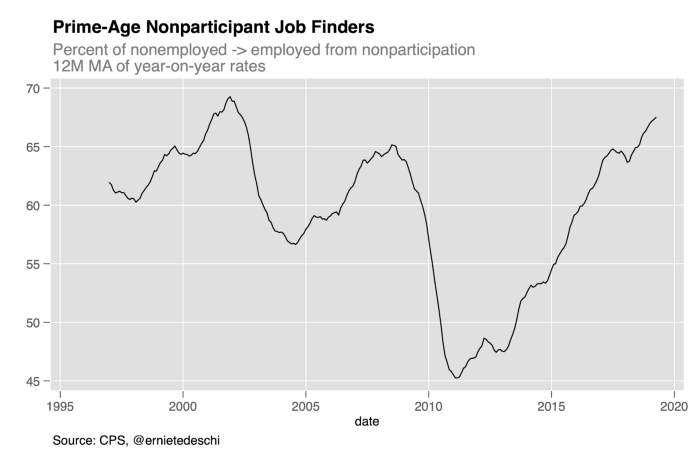
A broader notion of “maximum employment” that included more than just the unemployment rate would have shown that labor markets still had substantial room to run. In the late 2010s in particular, the relatively low unemployment rate also coincided with strong inflows directly into employment from the allegedly sidelined non-participants. The marginally slower pace of unemployment declines were almost perfectly matched by gains in labor force participation, showing that even “beyond full employment” more workers were willing and able to join the labor force as more jobs became available.

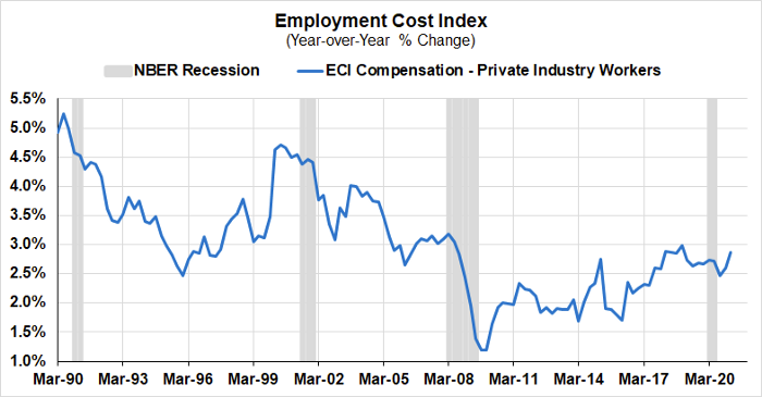
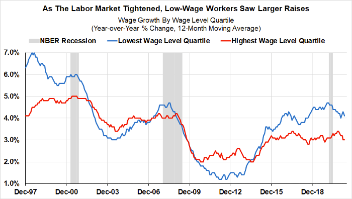
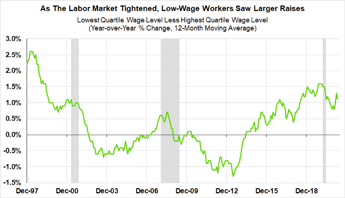
Even though aggregate wage growth was not as strong as the unemployment rate would have suggested, wages appeared to compress, with lower wage workers seeing outsized raises.

The ultimate lesson here is that estimates of “maximum employment” must shift as the capabilities of the economy grow and change. We know that the pre-pandemic labor market was not deeply inflationary, certainly not in any persistent way. But what we do not know is how much more room for endogenous improvement could have been achieved in the absence of the COVID-19 pandemic. Going forward, a reliance on upwardly sticky estimates of “maximum employment” risks leaving substantial gains in wages, employment, and economic growth on the table. While this is not an immediate risk as we exit the pandemic, understanding this point helps clarify the role that such assessments should play in both the Fed’s reaction function and policy goals.

2004–2006: Multi-Year Inflationary Dynamics May Imply Temporary Speed Limits, But Not Permanent Destination Limits

An approach that sheds the vestiges of Phillips Curve-based thinking will serve the Fed well as it looks to achieve maximum employment amidst more persistent — but not explicitly labor market driven — inflationary pressures. In our first piece in 2021, we highlighted the importance of wage and income dynamics, particularly as we move beyond reopening effects and one-time fiscal supports, to the inflation outlook. This view also aligns with our proposal for the Fed to adopt a framework that prioritizes the achievement of a floor rate of labor income growth. In fact, we have treated some of the peculiarities involved in the CBO’s use of the 2005 labor market as the definition of the “natural rate of unemployment” in detail. Today, a reprise of this scenario seems the most likely impetus to policy error as the reopening progresses: that inflation driven by temporary bottlenecks may prove a justification for policy tightening meant to cool off labor markets and curtail the recovery. To prevent this, the Fed’s “maximum employment” estimates should clearly communicate a distinction between near term and longer term employment goals, rather than abandon progress at the first sign of inflation.

Every economics textbook makes a distinction between “cost-push” and “demand-pull” inflation. On the cost-push side, supply constraints in certain commodities create inflationary pressures that won’t abate until capacity in those sectors expands, or the economy re-routes around them. Demand-pull inflation, by contrast, is usually attributed to increasing purchasing power among workers and households bargaining prices up. The “wage-price spiral” dynamic that most commentators cite as the paradigm case of inflation combines these two dynamics: higher wages mean households have more purchasing power to bid up prices and higher wages mean goods cost more to produce, creating, in theory, a persistent inflationary dynamic.

However, there is no reason every inflationary episode will have both sides of this dynamic. In fact, all else being equal, faster price increases reduce household surpluses and real income, thereby suppressing demand and curtailing future demand-side inflationary pressure. Even in the absence of policy tightening, the 1940s and 1950s show how even substantially larger inflation impulses than the Great Inflation can prove self-limiting. What both the 1970s Great Inflation, and the more recent experience of 2004–2006 show is that different inflationary dynamics should have different impacts on how we ought to assess “maximum employment.” Near-term inflationary pressures should not foreclose longer-term labor market goals.

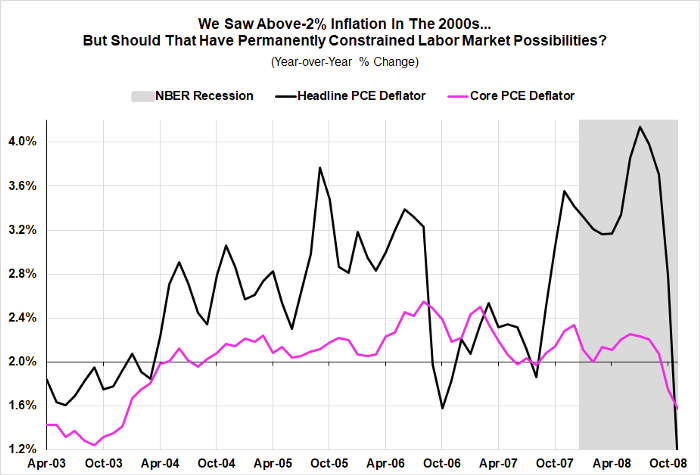
During the middle of the 2000s, both headline and core inflation readings ran persistently at or above 2% (headline and core PCE readings were ultimately revised up, showing more persistent overshooting). The Fed had not publicly adopted a formal 2% inflation target at that time, but leading Fed officials viewed the inflationary dynamics of that period as a basis for tighter policy. During this period, labor utilization had continued to make progress, while wage growth was sending mixed signals (average hourly earnings were accelerating from a slow rate, but the employment cost index was decelerating from a strong pace of wage growth).

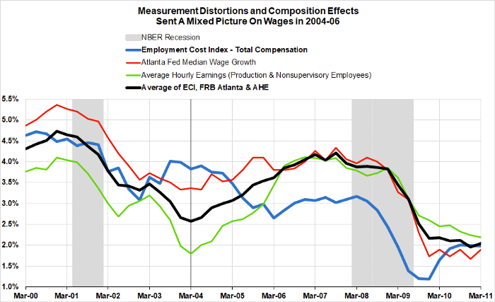
Amidst a decent US economy and a historically strong global economy, the primary driver of stronger inflation was commodity price inflation. Chair Bernanke dedicated multiple speeches to addressing and explaining the role this dynamic played in driving stronger inflation readings over this period. The strong demand amidst a historic global and emerging markets boom strained existing global capacity to produce several key commodities, including energy, food, and base metals. The time- and capital-intensive nature of capacity expansion in the production of energy and base metals necessarily implied a multi-year period of relevant cost-push pressures. Those pressures would show up most obviously in the food and energy components of inflation, but the fact that many of these commodities are at the absolute top of the supply chain for many goods meant inflation quickly bled through to the core components.

So, does this inflationary episode mean the period of 2004–2006 actually represented maximum employment? This is where some pedantry about the level of labor utilization versus the change in labor utilization proves most worthwhile. Certainly the Fed seemed to view the level of the unemployment rate during this period as the “natural rate of unemployment,” and held quite firmly to that view even a decade later when they over-tightened in the late 2010s. Yet while core inflation reared its head somewhat more persistently above 2% at approximately 5% unemployment in the mid-2000s, the same 5% unemployment rate did not yield the same inflationary results in the mid-2010s.

Ultimately, the inflationary constraint faced in 2005 was about capacity constraints in commodity production, not labor markets. Little understanding is added by any attempt to describe the situation with reference solely to the level of employment or labor utilization. The primary inflationary pressure was driven by commodity prices, not a feedback loop between prices and wages.

The timeline for developing additional commodity production capacity to meet domestic and global demand — and thus the timeline for the end of excess inflationary pressure — was also subject to substantial uncertainty. To tie this to our earlier narrative about the 1970s, oil prices would peak in the summer of 2008 and have one last hurrah in 2011 before global production met and surpassed global demand. With enough time for investment to respond to elevated commodity prices, new sources of production were developed that alleviated the source of persistent inflationary pressures.

A way to avoid this trap — the fear that the presence of inflation, regardless of cause, means that the economy has moved “beyond full employment” — is to instead look at the relationship between changes in labor utilization and changes in the price level (inflation). On this view, all-cause inflationary dynamics may indicate “speed limits” as to how quickly labor utilization can advance. However, these speed limits imply nothing about “maximum employment.” Labor markets can still make gains amidst inflation, but the pace of progress must be reconciled with the timeline for production capacity to feasibly catch up with current demand.

Luckily, the Fed’s new flexible average inflation targeting regime leaves open an additional degree of freedom for managing these dynamics, especially given the persistent constraints at the zero lower bound. By this, we mean that it may be worth allowing inflation to run moderately above 2% for some length of time if loose financial conditions are supporting the kind of capital spending and capacity expansion that will allow production to catch up with demand. Instead of clamping down on labor markets when capacity is expanding too slowly, the Fed’s new framework should allow them to give hesitant sectors a chance to invest in capacity without assuming the Fed will quickly cool the economy off again.

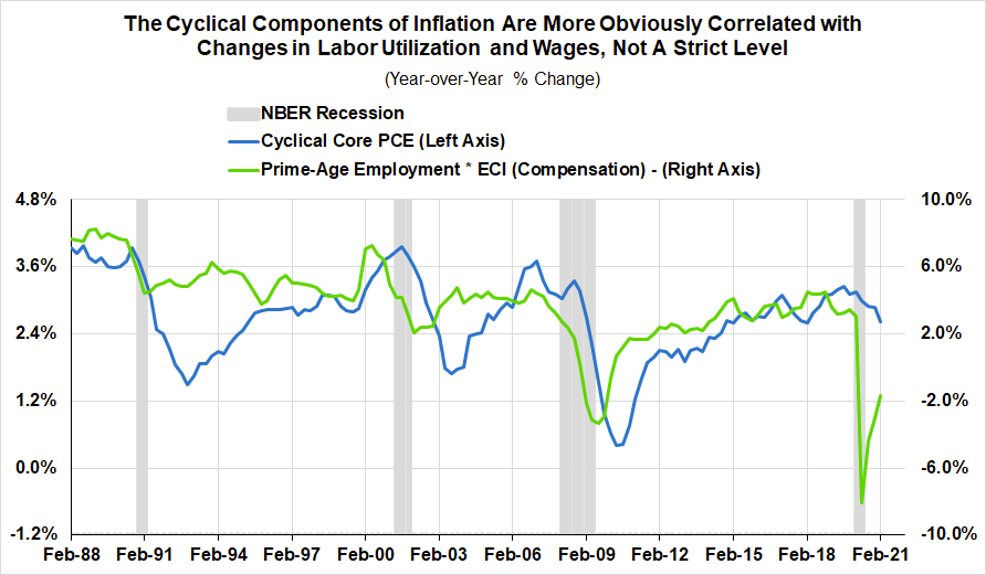
The alternative approach we suggest also fits the empirical and intuitive alignment of labor incomes with prices: why should a static level of labor utilization cause prices to increase persistently and more quickly? Data shows that trends in inflation, particularly trends in those components which are sensitive to business cycle conditions, are more obviously correlated to changes in labor utilization and wage incomes than they are to the level of labor utilization.

Instead, maximum employment assessments must be a moving target. Sometimes, like in 2016, that target can and should move quickly. Amidst signs of supportive income growth and persistent inflationary dynamics, that target might need to move more slowly or risk less manageable inflationary pressures. This, however, is no reason to decide ex-ante that there exists a permanent ceiling on the rates of labor utilization that can be achieved without undue inflation (cue cries that “it must be less than 100%!”).

This lesson is one of the most important when thinking about how robust estimates of “maximum employment” — especially the understanding that short-run inflationary pressures do not necessarily entail that labor markets have “overheated” — can inform better policy today. As the pandemic ends, and new bottlenecks are discovered in the supply chain, there is a real risk that some policymakers will use the inflation created by adjustment to a different demand environment as justification for abandoning labor market policy goals and tightening policy. However, as we explored at length with respect to the semiconductor industry, these shortages, and any inflation that may arise, are not a sign that workers “have it too good.” Rather, fiscal policy successfully supported consumer spending over the pandemic, and some firms and sectors are finally seeing sufficient demand to warrant investment for the first time in over a decade.

The trick now is to analyze where capacity constraints are causing problems, and target fixes for those problems. Hiking rates to throw people out of work will not do much to add capacity and sustainably resolve bottlenecks. As J.W. Mason and Mike Konczal argue, we must manage the boom and ensure targeted sectors get the investment and reforms they need to relieve capacity constraints while labor markets continue to make gains.

2009–2012: Resisting Recessionary Revisions That Conveniently Re-Classify Cyclical Employment Shortfalls

For a clever opponent, our call for a dynamic assessment of “maximum employment” might motivate symmetric demands for downward revisions the moment the current recovery slows. However, the Fed’s approach to labor market outcomes, the text of Section 2A of the Federal Reserve Act, and our own preferred framework make clear that “maximum employment” indicates a fundamentally asymmetric approach to demand management.

Demand-side policies should be actively addressing the fallout of painful recessions that inflict obvious cyclical dislocation. It is well within reason to aim for a labor market that proved feasible just 14 months ago.

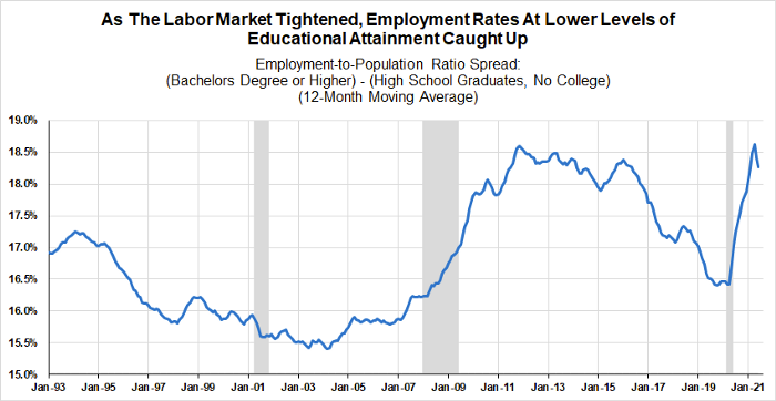
Historically, though, commentators and policymakers alike have often responded to long, slow recoveries by revising their estimates of “maximum employment” downwards. In this narrative — rather than demonstrating a failure to manage the business cycle — persistent unemployment following a recession instead indicates some “structural” mismatch preventing the economy from returning to pre-recessionary strength. If job loss can be reframed as “structural” rather than “cyclical,” it becomes the responsibility of workers to “find new skills” and “learn to code,” rather than the responsibility of policymakers to support workers through an economic downturn. Consider Charles Plosser’s claim in 2008 that unemployment would remain elevated simply because, “you can’t change a carpenter into a nurse.” This is not much different from the obsession with “skill-biased technological change” that gripped macroeconomists as the recovery dragged on past the two year mark. Unfortunately, this “structural” narrative can easily lead to premature policy tightening that stifles a nascent recovery.

You can see this clearly when looking at employment conditions by education level over the past fifteen years. In 2008, commentators were quick to declare workers without a college degree “structurally” unemployed in the new knowledge economy. Yet, as the recovery went on and labor markets tightened, these less-educated workers saw their employment rate outperform that of college graduates. Either these job losses were purely cyclical in the first instance, or the “knowledge economy” ended sometime in 2019.

As we have discussed at length, hard evidence of inflationary dynamics deserves to be treated on its own terms, not only through the lens of labor market dynamics. In the absence of such evidence, the Fed should continue to presume against downward structural shifts from the pre-pandemic labor market.

This presumption should be so strong that, to overcome it, we would need to see labor shortages translate into persistent wage-driven pressures that extend beyond one-time reopening effects. If there are more workers ready to be pulled in on the sideline, these dynamics should be fleeting if they appear at all. Anything short of such pressures starts to sound more like the anecdotal “labor shortage” and “structural unemployment” excuse-making of the prior recession.

Some may try to skirt this presumption by claiming that the Beveridge Curve — the borderline spurious relationship between a job openings rate and the unemployment rate — indicates that relatively high openings is prima facie evidence that workers’ existing capabilities are deficient. FOMC hawks used just this reasoning for premature policy tightening in the previous expansion. The expansion is vulnerable to similarly flawed extrapolations now, even though the Beveridge Curve approach elides the importance of recruitment intensity and ignores some basic empirical challenges. Job openings can outperform because of the technological ease of posting a job opening, and not necessarily because the opening represents a vacancy that a firm must urgently fill. It is not a surprise that estimated mismatches between job openings and the unemployed can follow relatively cyclical patterns.

The Conference Board’s failed attempt to reliably measure the quantity of online job openings reveals the importance of recruitment intensity when making any claims about the level of labor demand:

1. The internet is making it systematically easier to post more low-intensity openings for reasons independent of the business cycle, and
2. Job posting sites might actually raise the price of posting an opening when labor markets tighten, misleadingly reducing the quantity of observed openings when recruiting intensity ramps up.

As a wise man once said, to call a labor market hot, “you need to see some heat,” in the form of wage pressure. Job postings alone won’t cut it.

At this point in the recovery, there is still a real possibility that the “structural unemployment” narrative may take hold. Obviously, the timelines for returning to normal will look different across different sectors, but the goal of recovering obvious employment shortfalls should not. The critical benchmarks for assessing maximum employment should include a return to the pre-pandemic labor utilization (80.4% on the prime-age employment-to-population ratio) and the level of wages implied by the pre-pandemic trend (3% trend on the Employment Cost Index, ideally higher if we follow the parameterization of our preferred framework). Any less of a recovery should be considered an abdication of macroeconomic responsibility.

The Solution: Communicate The Dynamic and Multidimensional Nuances of Maximum Employment Assessments

As the pandemic ends, any of these three situations may tempt the Fed into a policy error. However, on the basis of the new framework and forward guidance, as well as statements from Chair Powell, this is not likely to be due to internal misunderstandings or misjudgments. FOMC members have reiterated their commitment to a broad understanding of “maximum employment” that goes far beyond the Phillips Curve.

However, the Fed faces a communication problem: markets and commentators have not fully internalized the new framework. Coverage has focused more obsessively on the implications of “flexible average inflation targeting” rather than on the asymmetric treatment of employment outcomes. The Fed is not providing enough information in the right structure to guide the public on what maximum employment can look like over time. This poses a problem, because the success of Fed policy is determined not just by their actions on monetary policy, but also by how private actors interpret their communications when pricing financial conditions under a variety of economic scenarios.

Without a clear view of what the Fed’s new labor market strategy means, the emergence of new economic conditions can spur substantial misalignment between the Fed’s intended policies and the public’s understanding of the Fed’s reaction function. It is ultimately the latter that determines the real economic impact of monetary policy. Ensuring that the Fed is able to make good on its new policy framework requires a change in communication.

The best way to do this, we think, is for the Fed to communicate its expectations for what values of multiple labor market indicators in the short and medium term qualify as realistic estimates for “maximum employment.” Like the SEP, these estimates should be subject to revision as new information is incorporated over time. In particular, the Fed should revise the SEP tables to include estimates of near-term “maximum employment” across a variety of metrics, to prevent markets from reading too much into a single indicator.

As a final note, adopting this strategy means the Fed must tread carefully to avoid an additional pitfall: that these estimates represent binding long-term values, and not interim targets and goals. As we have argued at length, the possibilities for “maximum employment” are dynamic, and change as the economy changes. By giving estimates for specific years, but not for a sui generis “longer run,” the Fed can help communicate to commentators and market makers that there is no ultimate, final point to labor utilization beyond which the economy cannot progress.

All of the scenarios we discussed amount to situations where the Fed, commentators or market participants decided, prematurely, that labor markets had reached the “longer run.” Each time, this led to narratives that further labor market progress was futile, and that the Fed should begin a tightening cycle to “normalize policy,” or the market would do it for them. By following, and properly communicating, the approaches outlined above, the Fed should be able to prevent a hijacking of its policy goals by more hawkish policymakers and market participants.

For those craving simple communication of Federal Reserve policy, this approach may annoy and confuse more than it enlightens, but “maximum employment” is a rich concept worthy of careful and iterative elaboration if the Fed is to fully follow through on its Congressional mandate, framework revisions, and forward guidance commitments. Most importantly, clear communication of its “maximum employment” goals will help the Fed avoid the policy mistakes of the past as the economy recovers from the ravages of the pandemic.